library(tidyverse)
library(skimr)Question 1
For Question 1, run the following R command to read the CSV file, spotify_all.csv as data.frame, spotify_all:
spotify_all <- read.csv('https://bcdanl.github.io/data/spotify_all.csv')rmarkdown::paged_table(spotify_all)The data.frame spotify_all includes information about Spotify users' playlists.
- The unit of observation in spotify_all is a track in a music playlist. 🎶
Q1a 🎶
Find the ten most popular song. 🎵
A value of a song is defined as a combination of a artist_name value and a track_name value.
Who are artists for those ten most popular song?
Q1a <- spotify_all %>%
  count(artist_name, track_name) %>%
  arrange(-n) %>%
  head(10)

Q1a
artist_name track_name n
1 Drake One Dance 143
2 Kendrick Lamar HUMBLE. 142
3 The Chainsmokers Closer 129
4 DRAM Broccoli (feat. Lil Yachty) 127
5 Post Malone Congratulations 119
6 Migos Bad and Boujee (feat. Lil Uzi Vert) 117
7 KYLE iSpy (feat. Lil Yachty) 115
8 Lil Uzi Vert XO TOUR Llif3 113
9 Aminé Caroline 107
10 Khalid Location 102Q1b 🎼
Find the five most popular artist in terms of the number of occurrences in the data.frame, spotify_all.
What is the most popular song for each of the five most popular artist?
Q1b <- spotify_all %>%
  group_by(artist_name) %>%
  mutate(n_popular_artist = n()) %>%
  ungroup() %>%
  mutate( artist_ranking = dense_rank( desc(n_popular_artist) ) ) %>%
  filter( artist_ranking <= 5) %>%
  group_by(artist_name, track_name) %>%
  mutate(n_popular_track = n()) %>%
  group_by(artist_name) %>%
  mutate(track_ranking = dense_rank( desc(n_popular_track) ) ) %>%
  filter( track_ranking <= 2) %>%   # I just wanted to see the top two tracks for each artist
  select(artist_name, artist_ranking, n_popular_artist, track_name, track_ranking, n_popular_track) %>%
  distinct() %>%
  arrange(artist_ranking, track_ranking)

Q1b
# A tibble: 10 × 6
# Groups: artist_name [5]
artist_name artist_ranking n_popular_artist track_name track_ranking
<chr> <int> <int> <chr> <int>
1 Drake 1 2715 One Dance 1
2 Drake 1 2715 Jumpman 2
3 Kanye West 2 1065 Gold Digger 1
4 Kanye West 2 1065 Stronger 2
5 Kendrick Lamar 3 1035 HUMBLE. 1
6 Kendrick Lamar 3 1035 DNA. 2
7 Rihanna 4 915 Needed Me 1
8 Rihanna 4 915 Work 2
9 The Weeknd 5 913 Starboy 1
10 The Weeknd 5 913 The Hills 2
# ℹ 1 more variable: n_popular_track <int>Q1c 🎹
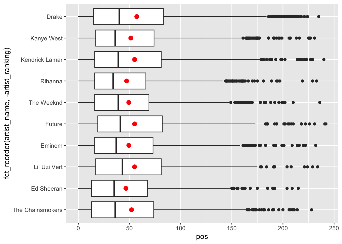
Provide both (1) ggplot codes and (2) a couple of sentences to describe the relationship between pos and the ten most popular artists.
Q1c <- spotify_all %>%
  group_by(artist_name) %>%
  mutate(n_popular_artist = n()) %>%
  ungroup() %>%
  mutate( artist_ranking = dense_rank( desc(n_popular_artist) ) ) %>%
  filter( artist_ranking <= 10)

# boxplot
ggplot(Q1c,
       aes(x = pos, y = fct_reorder(artist_name, -artist_ranking)) ) +
  geom_boxplot() +
  stat_summary(
    fun = mean,
    color = 'red'
  )
ggplot(Q1c) +
  geom_histogram(aes(x = pos), binwidth = 1) +
  facet_grid(fct_reorder(artist_name, artist_ranking) ~ .  , switch = "y") +
  theme(strip.text.y.left = element_text(angle = 0))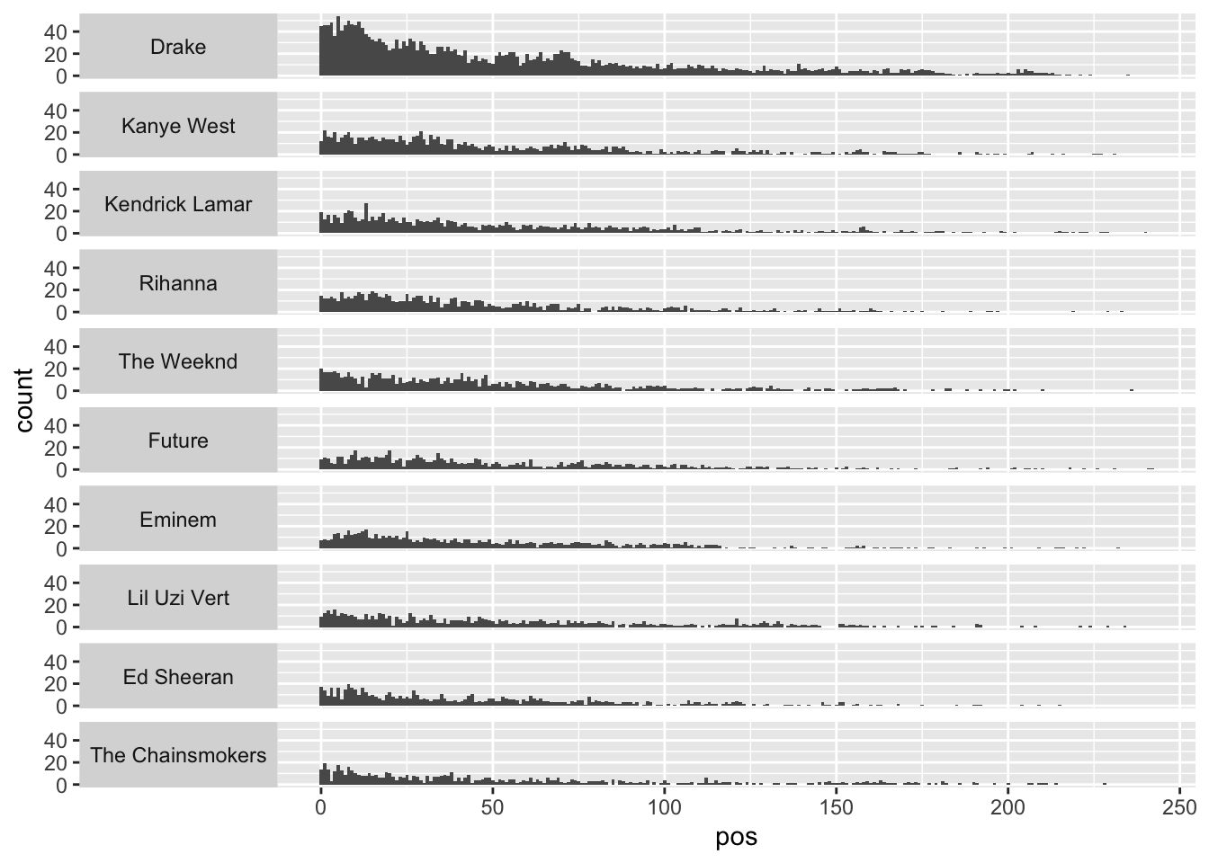
All are skewed right.
- Users tend to locate these popular artists' songs early in their playlist.
The distribution of pos does not seem to vary a lot across the ten most popular artists.
Anything noticeable can be mentioned.
Q1d 🎵
Create the data.frame with pid-artist level of observations with the following four variables:
pid: playlist id
playlist_name: name of playlist
artist: name of the track's primary artist, which appears only once within a playlist
n_artist: number of occurrences of artist within a playlist
Q1d <- spotify_all %>%
  count(pid, playlist_name, artist_name) %>%
  rename(n_artist = n) %>%
arrange(pid, -n_artist, artist_name)rmarkdown::paged_table(Q1d)